Why the Sci-Fi Quantum Computer Fails at the Weather

I recently read Der Zorn des Oktopus (“The Wrath of the Octopus”) by Dirk Rossmann and Ralf Hoppe, a novel in which a quantum computer is built to predict chaotic systems. The basic idea: determine weather events once it has “all the data”. If x is supposed to happen, a causal chain y has to occur first, and a sufficiently large quantum computer simply plays that chain forward. In the novel the machine is promptly abused to influence events: what has to happen so that event X takes place?

Reading this left me confused, because quantum computers, as they stand today, are not suited for this kind of computation. Yet the motif is popular in science fiction. Adam Fawer’s thriller Improbable has no quantum computer, but there someone turns into a so-called Laplace’s demon: an intelligence, conceived by Pierre-Simon Laplace in 1814, that knows the exact state of every particle in the universe and computes the entire future and past from it. The punchline: long before computing power becomes the issue, the demon fails at his input, because “all the data” is not something that physically exists (more on that below). So the half-sentence “once it has all the data” does not skip some minor detail, it skips exactly the spot where physics says no. Which made me ask, also because I had not followed the state of research for over ten years: are there quantum algorithms for chaotic systems at all, and where exactly does the idea break in practice?

The basic problem: linear versus nonlinear

A quantum computer computes in a fundamentally different way from a classical machine. Instead of bits (0 or 1) it works with qubits, which span huge state spaces through superposition and entanglement. The decisive catch for the weather scenario is the mathematics underneath: quantum mechanical time evolution under the Schrödinger equation is necessarily linear and unitary, probabilities are preserved.

The weather, however, is a highly chaotic system. Chaotic systems are deterministic and still unpredictable in the long run. They are described by nonlinear equations, such as the Navier-Stokes equations for turbulent flows or the simplified Lorenz model. Their defining feature is the butterfly effect: extreme sensitivity to initial conditions. If two initial states differ by as little as a millionth of a degree, their distance grows exponentially over time. This divergence is measured by the positive Lyapunov exponent. Even if the quantum computer were infinitely fast, the smallest measurement error in the input data blows up any exact trajectory prediction after a short time (the Lyapunov time).

So we are forcing a machine that only masters linear operations to solve a nonlinear problem. The currently most studied way to bridge this gap is called Carleman linearization.

Carleman linearization in one equation

The idea is old and elegant. You embed a nonlinear equation into a linear system by treating the powers of the variables as new, independent variables. The clearest way to see it is the simplest nonlinear example, the logistic equation:

Now define \(y_k := x^k\) and differentiate:

That is the whole mechanism. A nonlinear equation becomes a linear system, but one with infinitely many equations: \(y_1\) depends on \(y_2\), \(y_2\) on \(y_3\), and so on. In vector form this is \(\dot{\mathbf{y}} = A\,\mathbf{y}\) with an infinitely large, sparse matrix \(A\). And that is exactly the form a quantum computer likes: linear systems of differential equations can be handled by algorithms like HHL or newer linear solvers in time that grows only logarithmically with the dimension.

The catch: nobody can solve infinitely many equations. You truncate at some order \(N\) and set \(y_{N+1} = 0\). The last row then becomes \(\dot{y}_N = N\,y_N\), a pure growth term. The eigenvalues of the truncated matrix are simply \(1, 2, \dots, N\), all positive. Keep that in mind for a moment.

The experiment

How quickly this truncation breaks down is something an experiment can show. Here is the complete code: it solves the logistic equation exactly (analytically) and compares it with Carleman truncations of different orders, solved via the matrix exponential.

import numpy as np
from scipy.linalg import expm

def carleman_matrix(N):
    """Carleman matrix for dx/dt = x - x^2 with y_k = x^k.
    dy_k/dt = k*(y_k - y_{k+1}). Truncation: y_{N+1} = 0."""
    A = np.zeros((N, N))
    for k in range(1, N + 1):
        A[k-1, k-1] = k
        if k < N:
            A[k-1, k] = -k
    return A

def exact(x0, t):
    return x0 / (x0 + (1 - x0) * np.exp(-t))

def carleman_solve(x0, t, N):
    A = carleman_matrix(N)
    y0 = np.array([x0**k for k in range(1, N + 1)])
    return np.array([(expm(A * tt) @ y0)[0] for tt in t])

t = np.linspace(0, 1.6, 500)
x0 = 0.6
ex = exact(x0, t)
for N in [2, 4, 8, 16]:
    cl = carleman_solve(x0, t, N)
    err = np.abs(cl - ex)
    idx = np.argmax(err > 1e-2)
    print(f"N={N:2d}: breaks down at t={t[idx]:.2f}")

The result as a picture:

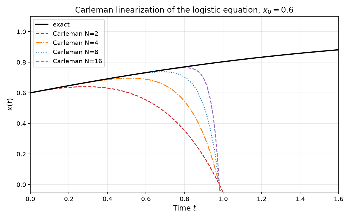
Two things stand out.

First: every truncation follows the exact solution perfectly for a while and then tips over abruptly. That is not a rounding error, it is structural. As soon as the truncated order becomes relevant, the growth term \(\dot{y}_N = N\,y_N\) from above takes over and the solution explodes. In the code you see maximum errors of \(10^{30}\) and beyond.

Second: higher order helps, but with clearly diminishing returns. Going from order 2 to 16, eight times the number of variables, only shifts the valid window from \(t \approx 0.2\) to \(t \approx 0.82\).

Why the window does not grow arbitrarily

The second point is the decisive one. There is a parameter that determines whether Carleman converges at all. Liu and colleagues showed in 2021 that the ratio \(R\) of nonlinearity to dissipative linearity decides the situation: for \(R < 1\) there is a genuine quantum advantage, for \(R \ge \sqrt{2}\) the problem is not efficiently solvable in the worst case¹. The logistic equation has a growing linear part instead of a damping one, so it sits deliberately in the hard regime, hence the early breakdown.

In fluid dynamics this \(R\) carries a familiar name. Several works link it to the Reynolds number, which measures precisely the ratio of inertial to viscous forces and thus how turbulent a flow is². Gonzalez-Conde and colleagues tie the convergence to the Kolmogorov scale, the grid resolution needed to resolve the energy cascade of the nonlinear term³. Sanavio and Succi get their lattice-Boltzmann-Carleman variant to work at moderate Reynolds numbers between 10 and 100 already at second order⁴. That is encouraging, but it does not describe real turbulence yet.

From the principle to real chaos: the Lorenz system

The logistic equation demonstrates the mechanism, but it is only one-dimensional and not chaotic. For a well-known chaotic system with several variables, consider the Lorenz system:

with the classic parameters \(\sigma = 10\), \(\rho = 28\), \(\beta = 8/3\). The system has three variables and shows real deterministic chaos with the famous butterfly attractor.

Carleman linearization works analogously: you define monomials \(x^a y^b z^c\) as new variables and derive the linear system in them. At truncation order \(N\) (all monomials with \(a+b+c \leq N\)) the dimension grows quickly: \(N=2\) needs 9 variables, \(N=3\) already 19.

Here is the code:

import numpy as np
from scipy.linalg import expm

def generate_monomials(N):
    """All monomials x^a y^b z^c with a+b+c <= N."""
    monoms = []
    for total in range(1, N+1):
        for a in range(total+1):
            for b in range(total+1-a):
                c = total - a - b
                monoms.append((a, b, c))
    return monoms

def deriv_monom(abc, sigma=10.0, rho=28.0, beta=8.0/3.0):
    a, b, c = abc
    terms = []
    if a > 0:
        terms.append((a * sigma, (a-1, b+1, c)))
        terms.append((-a * sigma, (a, b, c)))
    if b > 0:
        terms.append((b * rho, (a+1, b-1, c)))
        terms.append((-b, (a+1, b-1, c+1)))
        terms.append((-b, (a, b, c)))
    if c > 0:
        terms.append((c, (a+1, b+1, c-1)))
        terms.append((-c * beta, (a, b, c)))
    return terms

def carleman_matrix_lorenz(N, sigma=10.0, rho=28.0, beta=8.0/3.0):
    monoms = generate_monomials(N)
    idx = {abc: i for i, abc in enumerate(monoms)}
    n = len(monoms)
    A = np.zeros((n, n))
    for i, abc in enumerate(monoms):
        for coeff, abc_prime in deriv_monom(abc, sigma, rho, beta):
            if sum(abc_prime) <= N and abc_prime in idx:
                A[i, idx[abc_prime]] += coeff
    return A, monoms

def exact_lorenz_rk4(y0, t, sigma=10.0, rho=28.0, beta=8.0/3.0):
    def rhs(s):
        x, y, z = s
        return np.array([sigma*(y-x), x*(rho-z)-y, x*y-beta*z])
    states = [y0]
    dt = t[1] - t[0]
    for i in range(len(t)-1):
        s = states[-1]
        k1 = rhs(s)
        k2 = rhs(s + 0.5*dt*k1)
        k3 = rhs(s + 0.5*dt*k2)
        k4 = rhs(s + dt*k3)
        states.append(s + (dt/6)*(k1 + 2*k2 + 2*k3 + k4))
    return np.array(states)

def carleman_solve_lorenz(y0, t, N, sigma=10.0, rho=28.0, beta=8.0/3.0):
    A, monoms = carleman_matrix_lorenz(N, sigma, rho, beta)
    idx = {abc: i for i, abc in enumerate(monoms)}
    y0_carleman = np.array([y0[0]**a * y0[1]**b * y0[2]**c for a, b, c in monoms])
    states = []
    for tt in t:
        y_t = expm(A * tt) @ y0_carleman
        states.append([y_t[idx[(1,0,0)]], y_t[idx[(0,1,0)]], y_t[idx[(0,0,1)]]])
    return np.array(states)

# main run
y0 = np.array([1.0, 1.0, 1.0])
t = np.linspace(0, 2.0, 500)
ex = exact_lorenz_rk4(y0, t)
for N in [2, 3]:
    cl = carleman_solve_lorenz(y0, t, N)
    err = np.linalg.norm(cl - ex, axis=1)
    idx = np.argmax(err > 10.0)
    if idx == 0 and err[0] <= 10.0:
        print(f"N={N}: stable until t={t[-1]:.2f}")
    else:
        print(f"N={N}: breaks down (error > 10) at t={t[idx]:.3f}")

The result for the initial value \((1, 1, 1)\):

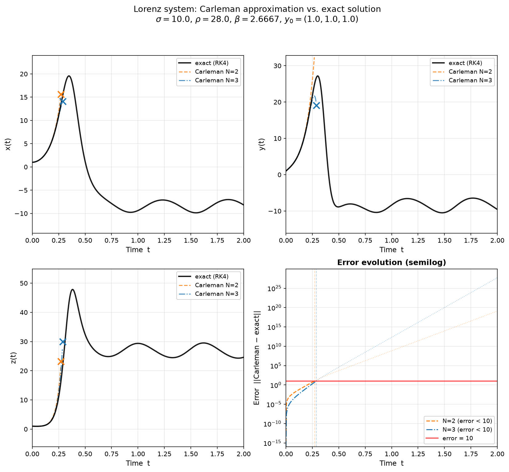
x(t), y(t), z(t) and the error on a log scale. The exact RK4 solution (black) stays bounded, the Carleman approximations (orange N=2, blue N=3) explode from t ≈ 0.3 on. The x marker shows the respective divergence point, the red line the error threshold of 10.

The difference to the logistic equation is drastic. Higher order barely helps here: from \(N=2\) to \(N=3\) the valid window only shifts from \(t \approx 0.27\) to \(t \approx 0.29\). For real chaos, the Carleman truncation is next to useless.

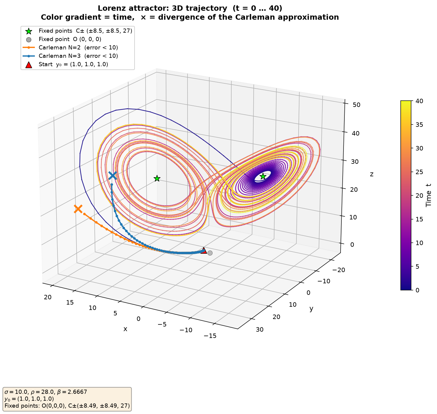
The exact trajectory forms the butterfly attractor, the color gradient encodes time. The Carleman approximations (orange N=2, blue N=3) follow only briefly and then diverge (x marker).

Fixable or fundamental

Still, the breakdown of the truncated Carleman matrix is not the final verdict on the quantum computer. By now there are workarounds such as pivot switching by Endo and Takahashi⁵ or pivot-shifted Carleman linearization⁶: you shift and rescale the system around a pivot state so that the truncated dynamics no longer inevitably diverges. The exploding matrix is primarily a numerical problem. For regular dynamics it can be defused.

The hard limit sits elsewhere. Lewis and colleagues proved in 2024 that any quantum algorithm that exactly propagates a system with a positive Lyapunov exponent has a complexity that grows at least exponentially with the simulated time⁷. That limit comes from the chaos itself; the Carleman truncation just happens to run into it first. Better code, pivot switching, or more qubits change nothing about it.

For the sci-fi plot this means keeping two things apart. The numerical breakdown of the Carleman method is a bug that clever people can fix. The exponential cost caused by chaos is a structural limit of the mathematics, not of the hardware.

A different line: quantum reservoir computing

The Carleman line tries to solve the differential equation itself. Since around 2023 a second route has established itself that reframes the problem. Quantum reservoir computing (QRC) uses the quantum system as a nonlinear substrate that approximates the attractor from a short observed time series. Only a classical readout layer is trained. The results are remarkable: Ahmed, Tennie and Magri predict extreme events in a turbulent shear flow model with correct timing using a recurrence-free variant⁸, Steinegger and Räth reproduce the short-term behavior and long-term statistics of eight prototypical chaotic systems with four qubits⁹, and Connerty and colleagues ran a quantum echo state network on real IBM hardware, far longer than the coherence times of the chip¹⁰.

What matters is what QRC cannot do. It approximates the attractor and delivers short-term forecasts, not a single trajectory over long horizons. The Lyapunov exponent strikes here just the same, without Carleman and without truncation. QRC shows that quantum computers can indeed take over a certain prediction task. It is just not the one the novel promises: the exact future from complete initial data.

Getting the data in and out

The half-sentence “once it has all the data” hides an assumption that is easy to miss: that the data can get into the machine at all. Algorithms of the HHL family deliver their exponential speedup only if the input is already available as a quantum state. Loading trillions of classical sensor readings into the amplitudes of a quantum register is the state preparation problem, and the standard answer to it, a quantum random access memory (QRAM)¹¹, exists essentially on paper: the circuits it requires are deep and error-prone, and nobody has built one at scale. Aaronson pointed at exactly this fine print years ago: if loading the data costs as much as solving the problem classically, the quantum advantage evaporates¹². So the sci-fi computer does not fail at the computation first, it fails at the loading dock, and by the time the state is prepared, the weather has moved on.

The other end is not free either. If the algorithm produces a quantum state that encodes the solution field, a measurement collapses it and yields only a limited amount of classical information per run. For an expectation value that is fine, for a complete weather field it is not. To be fair, the QRC line has learned to work around the collapse where it hurts most: weak measurement protocols read the reservoir gently enough that the computation can keep running¹³, and feedback-driven QRC performs projective measurements but feeds the results straight back into the circuit as new rotation angles, keeping the memory of the system alive¹⁴. Both tricks keep a running forecast going. Neither hands you the full solution vector of a differential equation.

And then there is the initial data itself. Chaos means sensitive dependence on initial conditions: \(\delta(t) \approx \delta(0)\,e^{\lambda t}\) with a positive Lyapunov exponent. To predict \(T\) time steps ahead you need roughly \(\lambda T\) additional bits of precision in the input. This holds for every computer, classical or quantum. “Having all the data” does not physically exist.

This is exactly the premise Laplace’s demon already hangs on. The demon could own perfect instruments and still fail: the required precision grows without bound with the forecast horizon, so “all the data” would have to mean arbitrarily many decimal places. The premise breaks classically, no quantum mechanics required. With that, the foundation of “once it has all the data” is gone, with or without a quantum computer.

Conclusion

Back to the original question: are there quantum algorithms for chaotic systems, and where does the novel’s idea break? They exist, and they are an active field of research, with Carleman linearization as the common thread. But the gap between “can efficiently simulate other quantum systems” and “predicts the weather once it has all the data” does not hang on the hardware. It hangs on two mathematical facts: linear time evolution meets nonlinear chaos, and the initial conditions would require a precision that does not physically exist. Both are structural, and structure does not yield to better hardware. On top of them sit the practical barriers at both ends, loading the data without a QRAM and reading the solution out through measurements: those are engineering, but engineering nobody has done.

That is also what makes the novel’s idea interesting: it points at real research, but the half-sentence “once it has all the data” quietly defines both problems away. The experiment above makes the first one visible, the second sits in a single exponential function. An afternoon of code is enough to make a whole novel’s premise wobble.

Sources